An AI agent ran an IBNR reserve analysis on a healthcare claims dataset. Five thousand three hundred twenty-six claims. Nine accident years. One data file.
The agent analyzed it four times.
Four different IBNR estimates. The lowest was $46 million. The highest was $98 million. The spread between them was $51 million, which is 110 percent of the lowest estimate. Same data, same prompt, same instruction to apply the chain-ladder method. Four answers that cannot all be right.
The problem is not that one of those answers is wrong. The problem is that any of them could have been the number an actuary submitted, and nothing in the output would tell you which one to trust.
This is the fifth experiment in a series testing whether the delivery mechanism for knowledge affects how AI agents make structured professional decisions. The previous experiments covered claim adjudication, clinical triage, financial due diligence, and prior authorization. Each found that flat-document agents produced errors that decision trees eliminated, and that better models would not close the gap. This experiment finds something different in structure but identical in cause. IBNR reserve estimation does not have a right or wrong output the way a coverage decision does. It has a methodology. When the methodology is delivered as a flat prompt, the agent fills in the gaps differently on every run. When it is delivered as a decision tree, the gaps do not exist.
The Domain
IBNR stands for Incurred But Not Reported. It refers to claims that have occurred but have not yet been submitted, processed, or fully paid at the time of valuation. Every insurer carries an IBNR reserve on its balance sheet, representing its best estimate of what it will eventually owe on events that have already happened.
The chain-ladder method is the standard approach to estimating that reserve. An actuary builds a triangle: rows are accident years (the year a loss occurred), columns are development lags (how many years after the accident year the payment was made). Each cell is the cumulative amount paid for that accident year through that lag. The triangle is incomplete by construction. Recent accident years have only a few observed columns. The chain-ladder method fills in the missing cells by computing age-to-age development factors from the completed diagonals and applying them forward.
The method is well-defined in its mathematics. What it does not pin down is a sequence of construction choices that precede the mathematics, choices that look like minor implementation details but that determine the answer.
The Three Decisions That Create Variance
Handed a raw claims file and told to run a chain-ladder analysis, an AI agent must make at least three decisions before it touches a single development factor.
How to define development lag. A typical definition is: paid calendar year minus accident year, as a plain integer. A claim incurred in 2008 and paid in 2011 belongs in lag 3. A claim paid in its accident year belongs in lag 0. An agent that computes lag differently, counting months instead of years, or adding 1 to convert from zero-indexed to one-indexed, produces a differently shaped triangle with different row counts and different LDFs. The same underlying data produces structurally different inputs.
How to handle the triangle boundary. Each accident year has a natural cutoff: the latest year in which payments were observed. Beyond that cutoff, the cell is empty. An agent that fills empty cells by repeating the last observed value treats every accident year as fully developed past its observed lag, which understates the remaining LDFs and compresses the reserve. An agent that leaves those cells blank correctly identifies each accident year's maturity date and applies the appropriate factors forward.
Whether to apply a tail factor and a BF adjustment for immature years. The chain-ladder method projects the most recent accident years using development factors estimated from more mature years. For accident years that are only 30 or 60 percent developed, that projection is highly sensitive to the selected factors. The Bornhuetter-Ferguson method blends the chain-ladder projection with an independent a priori estimate, reducing the leverage effect. Similarly, the tail factor accounts for development beyond the last observed transition. An agent that uses pure chain-ladder for all years and sets the tail to 1.000 produces a different answer than one that applies BF to immature years and derives the tail from the decay pattern in the last three LDFs.
Each of these decisions is documented in actuarial practice. None of them is resolved by telling the agent to use the chain-ladder method. That instruction is necessary but not sufficient. The remaining choices determine the answer.
The Setup
The dataset is a healthcare claims file: 5,326 rows covering accident years 2005 through 2013, with claims paid through December 2013. The file contains three fields: incurred date, paid date, and claim amount.
The flat prompt. A single prompt instructing the agent to perform a chain-ladder IBNR analysis using the data, report IBNR as a percentage of ultimate, and write results to a timestamped file. No lag definition. No guidance on triangle boundary handling. No specification of tail or method. Four independent runs.
The expertise tree. The same analysis framed as a seven-node decision tree in mcpforx, a platform that delivers structured expertise to AI agents through MCP. The tree pins every construction decision explicitly. Node 2 defines development lag to the character: paid calendar year minus accident year as a plain integer, with examples. It states that cells beyond the last observed lag must remain empty, not carry forward. Node 4 derives the tail factor from the decay ratio of the last three LDFs and applies a capping rule. Node 6 assigns BF to any accident year below 70 percent developed and derives the a priori from reference years above 85 percent. The agent follows the tree step by step using find_expertise and next_step calls. Four independent runs.

Results
Flat Prompt (4 runs)
Range: $46M to $98M. Spread of $51M.

Expertise Tree (4 runs)
Range: $107.36M to $107.38M. Spread of $17,752, which is 0.017 percent.
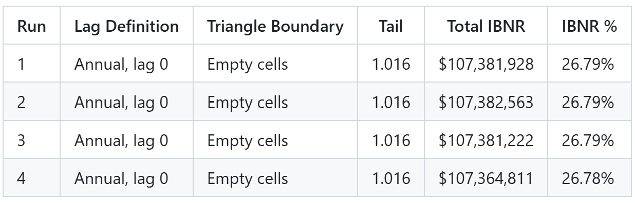
The tree runs differ from each other by floating-point rounding in the Python calculations. They are, for any practical purpose, the same number.
What Each Decision Contributed
The Triangle Boundary
The most consequential error across the flat runs was the carry-forward bug. When an agent groups paid amounts by (accident year, development lag) and then takes the cumulative sum, empty cells in the source group become zeros. Cumulative-summing over zeros repeats the last observed value across all remaining columns. The result is a triangle where every accident year appears fully developed at every lag, because each row ends with the same number repeated as far as the columns extend.
When LDFs are computed from this triangle, they reflect true development in the columns where actual payments occurred, but are pulled toward 1.000 in the columns where zeros have been silently added. When each accident year's maturity is identified by finding the last cell with a non-zero value, the result is the last column in the matrix, which for every accident year is the maximum lag. The agent concludes that AY2013 is as mature as AY2005 and projects forward a distance of zero. It is not hallucinating. It is computing correctly from a triangle it built incorrectly.
Runs 2, 3, and 4 all produced this bug. Run 1 avoided it by using monthly development periods, which produced a different kind of structural error instead: a 96-period triangle where AY2013 had only 12 observed months against a full tail computed from 96-month patterns.
The Tail Factor
All four flat runs set the tail to 1.000, meaning no development is projected beyond the last observed transition. The tree derived the tail from the decay pattern in the last three LDFs: 1.0472, 1.0294, 1.0218. The decay ratio is 0.742. The raw tail LDF is 1.0162. Capped to three decimal places: 1.016. Applied to the most mature accident year, AY2005 at 98.4 percent developed, this adds $405,344 in IBNR to a year that flat runs treated as closed.
The tail is small in absolute terms for the mature years. Its compounding effect on less developed accident years is larger. And its absence is a choice the flat prompt agents made without acknowledging they were making it.
The BF Adjustment
This is the decision with the most dollar impact. AY2013 at valuation date was 29.9 percent developed. Under pure chain-ladder, that accident year's ultimate equals its lag-0 paid amount of $17.1 million multiplied by its CDF of 3.34, which yields approximately $57 million. Under Bornhuetter-Ferguson, the IBNR component is derived from an a priori expected ultimate rather than from observed paid alone, reducing the leverage effect of applying a high CDF to a small base.
None of the flat runs applied BF. The tree applied it to AY2012 (60.4 percent developed) and AY2013 (29.9 percent developed). For AY2013 specifically, the BF treatment contributed $42 million of the tree's total $107 million reserve. The flat runs either collapsed AY2013 to zero additional development (carry-forward) or applied pure chain-ladder to a year that was less than one-third developed.
The BF method exists precisely because pure chain-ladder is unreliable for immature accident years. An actuary who applied pure chain-ladder to a year with 30 percent maturity and signed the reserve would be departing from standard practice. The flat prompt agents did not know they were doing this. The tree knew they shouldn't.
The Variance Is the Failure
In the previous experiments in this series, the flat-document agent produced a wrong answer. A claim was denied that should have been approved. A triage level was assigned incorrectly. The error was detectable against a known correct answer.
IBNR estimation does not work that way. There is no observable correct answer at the time of analysis. The reserve will prove adequate or inadequate when claims eventually develop to their true ultimate. Until then, all you have is the method and the number it produces. An actuary reviewing a single run of the flat prompt would find an answer that looks reasonable: a percentage of ultimate, a development pattern, a set of LDFs. The output format does not reveal whether the triangle was constructed correctly. It does not flag that the tail was set to 1.000 by default. It does not indicate whether BF was considered.
Run the analysis four times and the range from $46 million to $98 million becomes visible. Run it once, as you would in production, and you have a number with no indication of how sensitive it is to the choices that produced it.
The tree runs ranging from $107.364M to $107.382M are not just more consistent. They are consistent because the methodology was specified rather than inferred. An actuary reviewing tree run output sees: lag definition, triangle construction rule, tail derivation formula with inputs, method assignment by accident year, a priori derivation method. The number can be audited against the choices that produced it. The flat prompt number cannot.
This matters because IBNR reserves are line items on audited financial statements. Actuaries are credentialed professionals who certify their work. The certification is not just of the number, it is of the methodology. A model that applies inconsistent methodology across runs without disclosing that inconsistency is not an actuarial tool. It is a spreadsheet that changes its formulas between saves.
Tradeoffs
The tree approach takes more effort to build than a prompt. Every decision in the methodology had to be made explicit during construction rather than left to the agent. That work is front-loaded and requires domain expertise. An actuary has to sit down and specify, in node instructions, exactly what lag means, exactly how to handle the triangle boundary, exactly how the tail derivation works. The prompt requires none of that.
The latency is higher. Seven sequential MCP calls with Python scripts running at each step adds clock time that a single flat run avoids. For a single analysis this is negligible. For high-volume automated reserve work, it compounds.
The tree is also bounded by its design. The hybrid CL/BF approach encoded in this tree is one methodology. A run that required different segment handling or a different a priori basis would require the tree to be extended. The flat prompt adapts to whatever the agent infers from context. That flexibility is also its failure mode.
Against all of this: a $51 million range on a single dataset. If the flat prompt ran once and produced $46 million and that number went into a financial statement, the question is not whether it was close enough. The question is whether anyone would have known it might have been $98 million instead.
Conclusion
Four flat prompt runs on the same healthcare claims data produced IBNR estimates of $46 million, $54 million, $97 million, and $97 million. The variance traced to three construction choices the agents made differently across runs: lag definition, triangle boundary handling, and method assignment for immature accident years. No run disclosed what choices it had made. No run acknowledged the choices were choices.
Four tree runs produced $107.38M, $107.38M, $107.38M, and $107.36M. The difference between the best and worst tree run is less than eighteen thousand dollars on a hundred-million-dollar reserve. The methodology is auditable at every node. The number is reproducible.
The flat prompt approach is not wrong because the agent is careless. It is wrong because estimating reserves from raw claims data requires a sequence of methodology decisions that the method's name does not resolve. Chain-ladder is not a single algorithm. It is a class of algorithms distinguished by construction choices. Telling an agent to use chain-ladder and leaving those choices unspecified is the actuarial equivalent of telling a surgeon to operate and leaving the technique to their discretion. The discretion is the problem.
A model that knows what chain-ladder means will always produce some answer. The answer will always look like an IBNR estimate. It will always be presented with appropriate precision and appropriate format. Whether the methodology behind it is reproducible is not visible in the output. Whether it matches what a credentialed actuary would certify is not visible in the output. Whether the same model would produce the same number tomorrow is not visible in the output.
Structure makes it visible. The tree makes methodology decisions before the model arrives and records them in the run trace. The investment is human expertise encoded once. The return is methodology that does not change between runs.
MCPforX.com is a platform for building and deploying structured expertise as MCP-accessible decision trees. The claims data is a synthetic healthcare dataset. Full run traces and result files are available on request.